Eddy Heat Transport
Middle latitude weather systems are the primary mechanism of poleward heat transport. See an example of observed eddies stirring the N-S temperature gradient – 850 mb Temperature loop.
The meridional heat flux due to transient eddies is defined by
We can plot these data from analyzed fields as follows, using the ERA5 Reanalysis dataset.
Instructions for plotting transient heat fluxes from ERA5 reanalysis:
1. Download the following zipped folder poleward_transient_energy_flux that contains:
- ERA5 Data (netcdf file) for yearly mean transient poleward heat and moisture flux
- Matlab/Python script that will read in the netcdf file, manipulate the data, and plot figures. You need to follow the instructions in the code. There is a utility file to plot coastlines in Matlab (coast.m). You do not need to modify this utility file, but make sure all files are in the same folder.
2. The first two options in the script will plot the transient heat flux for individual layers and averaged in the vertical (see figures in the examples below). You will need to modify the script to calculate and plot zonally averaged transient heat fluxes and vertically and zonally integrated transient energy flux.
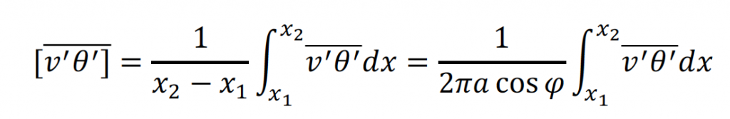
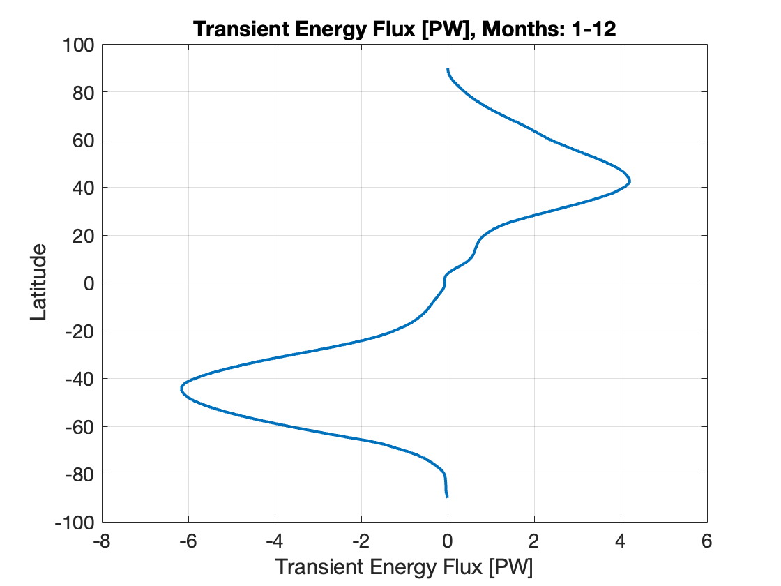
The net northward heat flux by transient eddies is given by
Here, a is the Earth radius, φ is the latitude and we have used hydrostatic balance to express the rhs as an integral in pressure.
Note: The zonal average of the transient heat flux is calculated using-
4. Use your plots and the equations above to estimate the net northward transport of heat at a chosen latitude of 45°N. Compare your estimate with the atmospheric heat transport derived from Earth radiation budget-
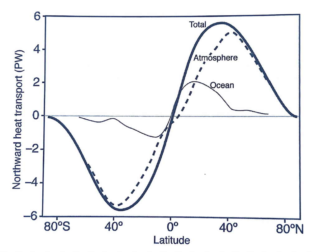
Figure: The ocean (thin) and atmosphere (dotted) contributions to the total northward heat flux based on NCEP Reanalysis (Trenberth and Caron, 2001). The units of heat transport are in PW (1015 W).
Transient Meridional Heat and Energy Flux
Your analysis should produce the following figures (shown below):
- The 850 hPa level meridional heat flux (in units of K m s-1 )
- The vertically averaged heat flux (in units of K m s-1 )
- The zonally averaged heat flux (in units of K m s-1 )
- The zonally and vertically integrated energy flux, respectively (in PW)
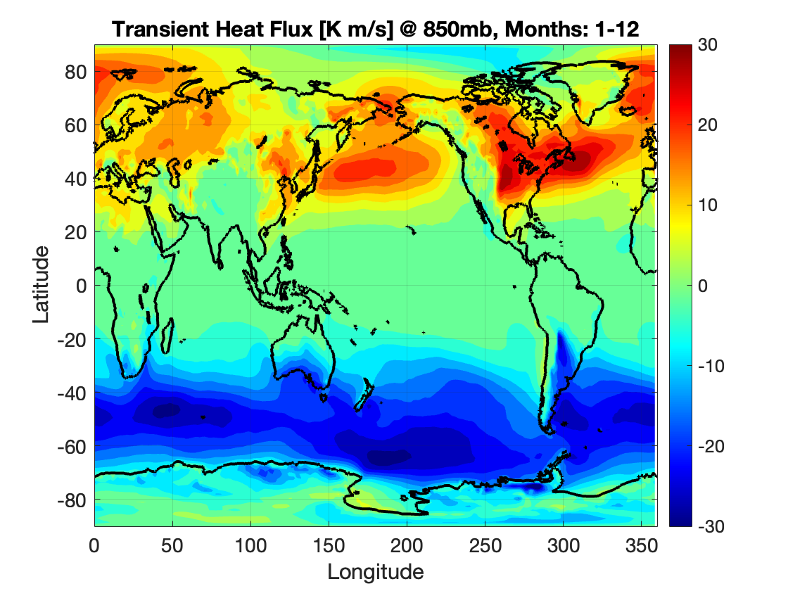
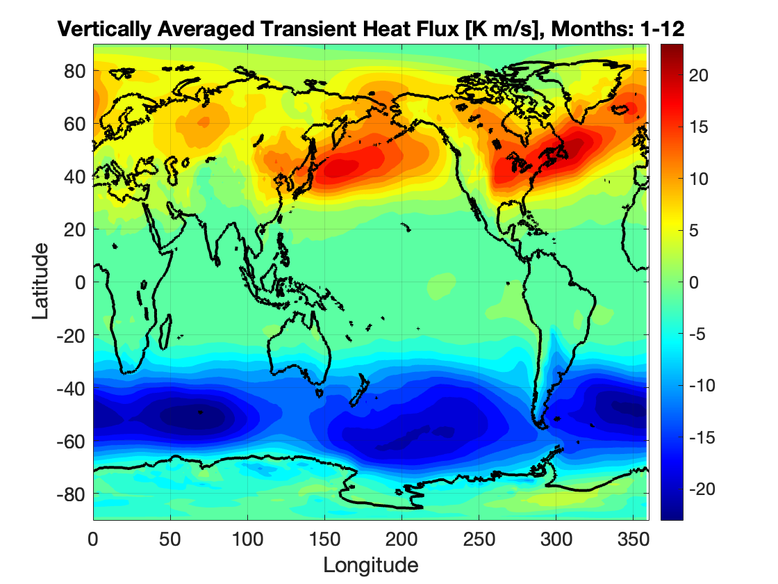
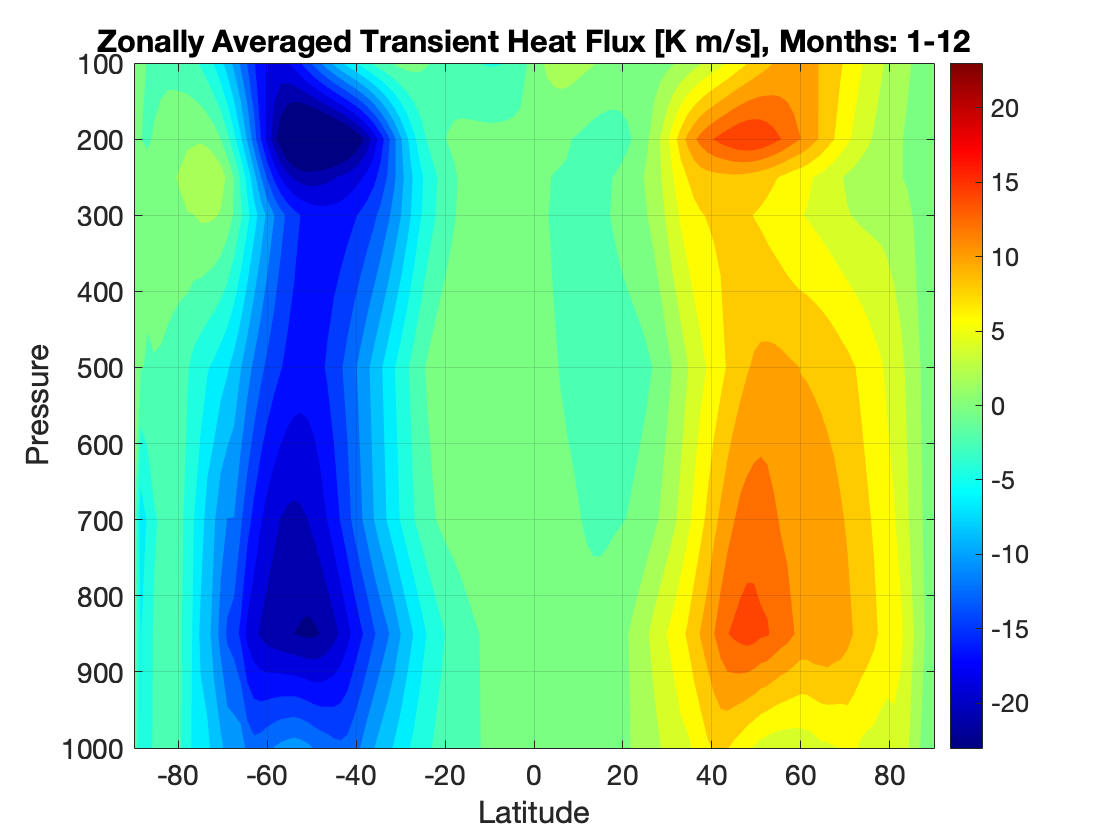
Note that the regions of highest meridional heat transport are located at about 45N and correspond to the middle-latitude storm tracks. The largest transport occurs in the Pacific and Atlantic Oceans, directly downstream of continents. Additionally, there are two local maxima in the vertical profile, one at 850 mb (the top of the atmospheric boundary layer), and another at 200 mb (the region of strongest jet).